3D Object Reconstruction Via Inverse Rendering
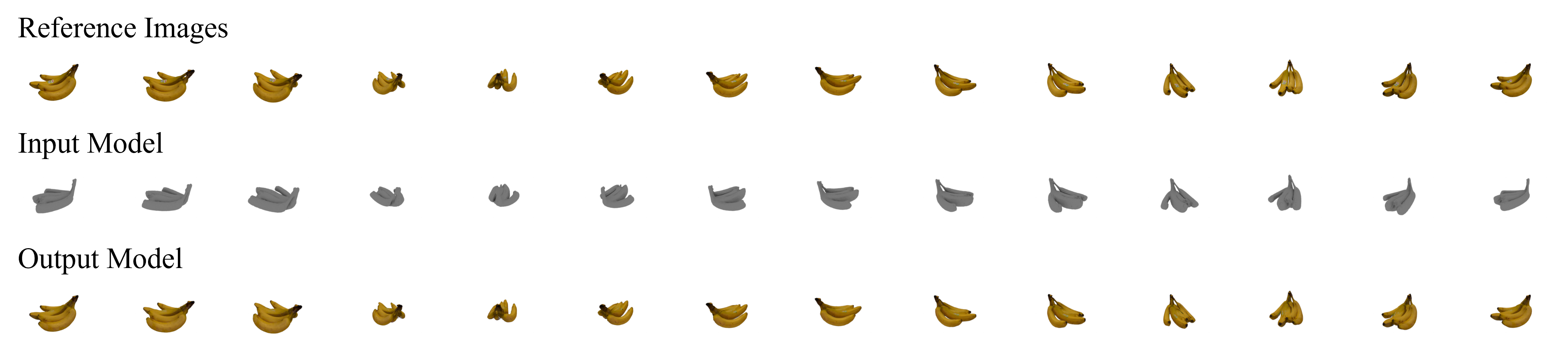
A practical pipeline that combines camera pose estimation, interactive segmentation, single-image reconstruction, and differentiable rendering to recover a textured 3D object from a sparse set of photographs.
Turning a few photographs into a convincing 3D object sounds straightforward: find the object in each image, infer its shape, and add a texture. In practice, every part of that sentence hides an ambiguity. The cameras are unknown, the background contaminates the reconstruction, and many different shapes can explain the same set of pixels.
For our final project in Yale’s CPSC 579: Advanced Computer Graphics, Andrew Yi and I built a pipeline that tackles those ambiguities in stages. It combines COLMAP for camera pose estimation, SAM 2 for foreground segmentation, TripoSR for a coarse single-image mesh, and Mitsuba 3 for differentiable inverse rendering.
The central idea is simple: do not ask inverse rendering to discover an object from nothing. Give it an approximate shape with the right topology, then let evidence from all available views refine both the geometry and its appearance.
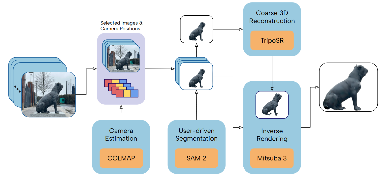
Figure 1: Our reconstruction pipeline. Each stage reduces a different source of ambiguity before the final optimization.
Why a staged pipeline?
Classical structure-from-motion and multi-view stereo are excellent when they receive many sharp, well-textured photographs with strong overlap. Casual object captures are less cooperative: there may be only a handful of views, the background may dominate the feature matches, and smooth or reflective surfaces provide few reliable correspondences.
Learning-based single-image reconstruction has the opposite trade-off. It can produce a plausible complete object from one photograph, but the unseen side is necessarily an informed guess. Inverse rendering can reconcile a model with several observed views, yet it is an under-constrained optimization problem and is highly sensitive to its starting point.
Our pipeline assigns each subproblem to the tool best suited to it:
- Recover camera intrinsics and poses from the original photographs.
- Remove the background with a promptable segmentation model.
- Infer a complete, watertight coarse mesh from one strong object view.
- Align that mesh with the recovered cameras.
- Jointly optimize mesh vertices and vertex colors against every selected photograph.
We exposed the early stages through a small desktop interface. The components were implemented as separate Python engines, which made it easier to test each one independently and swap methods during development.
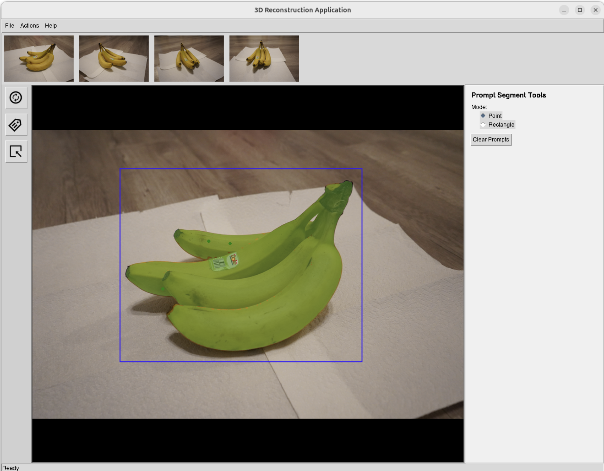
Figure 2: The prototype interface for loading photographs, generating masks, estimating cameras, and producing the initial mesh.
Step 1: recover the cameras
Inverse rendering only works if a rendered pixel and its reference pixel describe the same ray through the scene. A small camera-pose error gives the optimizer contradictory instructions: moving the surface to satisfy one view makes it disagree with another.
We use COLMAP’s incremental structure-from-motion pipeline to extract up to 8,192 RootSIFT features per image, perform exhaustive matching with geometric verification, and jointly estimate the cameras and a sparse point cloud. The output gives each image an intrinsic matrix (K_i), rotation (R_i), and translation (t_i).
We then import the reconstruction into Blender to inspect the camera arrangement and align the object. The scene is exported through the Mitsuba Blender add-on, converting COLMAP’s camera estimates into Mitsuba sensor transforms.
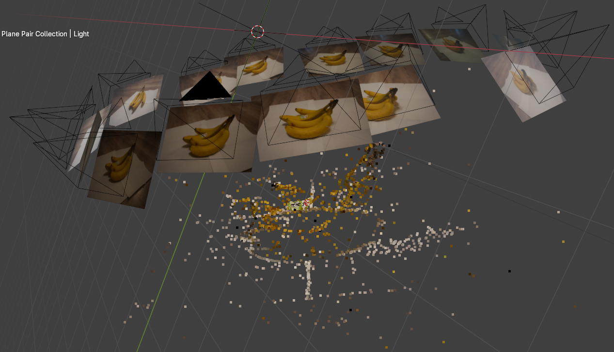
Figure 3: Recovered cameras and sparse COLMAP reconstruction visualized in Blender.
Step 2: isolate the object
A reconstruction model should not have to decide whether the table, wall, or shadow belongs to the object. We use SAM 2 to create a binary foreground mask from positive and negative clicks or a bounding box. Simple morphological cleanup removes small holes and isolated regions, and the result is exported as a transparent-background crop.
User guidance proved more practical than relying entirely on automatic masks. A single deliberate prompt is fast, and it resolves ambiguities—such as a banana touching its shadow—that an automatic mask generator may interpret differently.
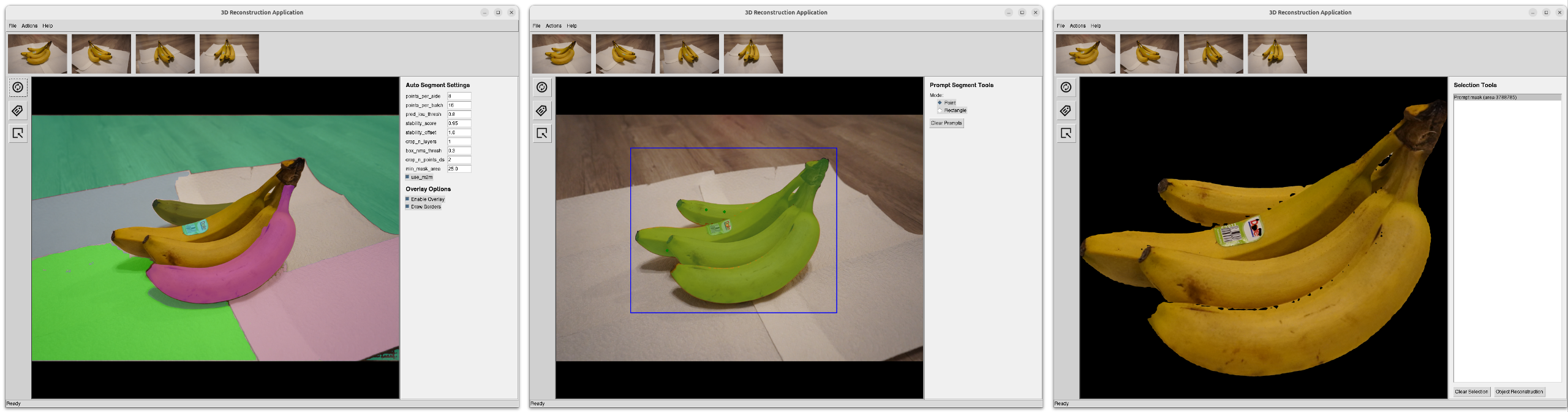
Figure 4: A user prompt produces the mask used to remove the background before reconstruction.
Step 3: build a coarse geometric prior
One masked view is passed to TripoSR, which predicts a latent scene representation and evaluates it as a signed-distance field on a (256^3) grid. Marching Cubes extracts the zero level set as a watertight triangle mesh. The network can also unwrap the mesh and bake its predicted colors into a texture atlas.
This first mesh is not expected to be exact. Its job is to place vertices near the correct surface and, more importantly, to provide a useful topology. For our banana test object, the difference between a mesh that separates the individual bananas and one that fuses them together determines what the later optimizer can recover.
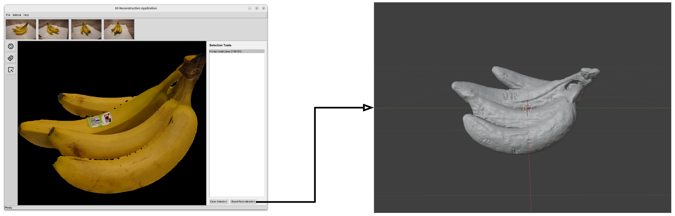
Figure 5: From a segmented photograph to TripoSR’s coarse textured mesh.
Step 4: refine shape and appearance with inverse rendering
Ordinary rendering maps scene parameters to an image. Inverse rendering runs that process backward: it adjusts scene parameters until rendered views resemble the photographs.
For each training view, Mitsuba renders the current mesh, compares it with the matching reference image, and differentiates the image-space error with respect to the model. We optimize two parameter groups together:
vertex_positions, using Mitsuba’s large-steps geometry optimization, controls the shape;vertex_colorcontrols the spatially varying appearance.
With rendered image (\hat I_i), reference image (I_i), and the set of selected views (\mathcal V), our objective is the L1 pixel loss
We downsample the original 6000 × 4000 photographs to 600 × 400 for optimization, use Adam with a learning rate of 0.01, and run for 100 iterations. In our experiments, the loss generally stabilized after 60–80 iterations.
Results: six views versus fourteen
We photographed a bunch of bananas from 14 directions and generated the initial mesh from view 11. With only six reference views, the optimizer already produced a recognizable model that remained plausible from withheld angles. Using all 14 views improved fine geometry and image similarity, although the region between the two central bananas still revealed missing coverage. A top-down photograph would likely have constrained that area better than simply adding more views around the same horizontal arc.
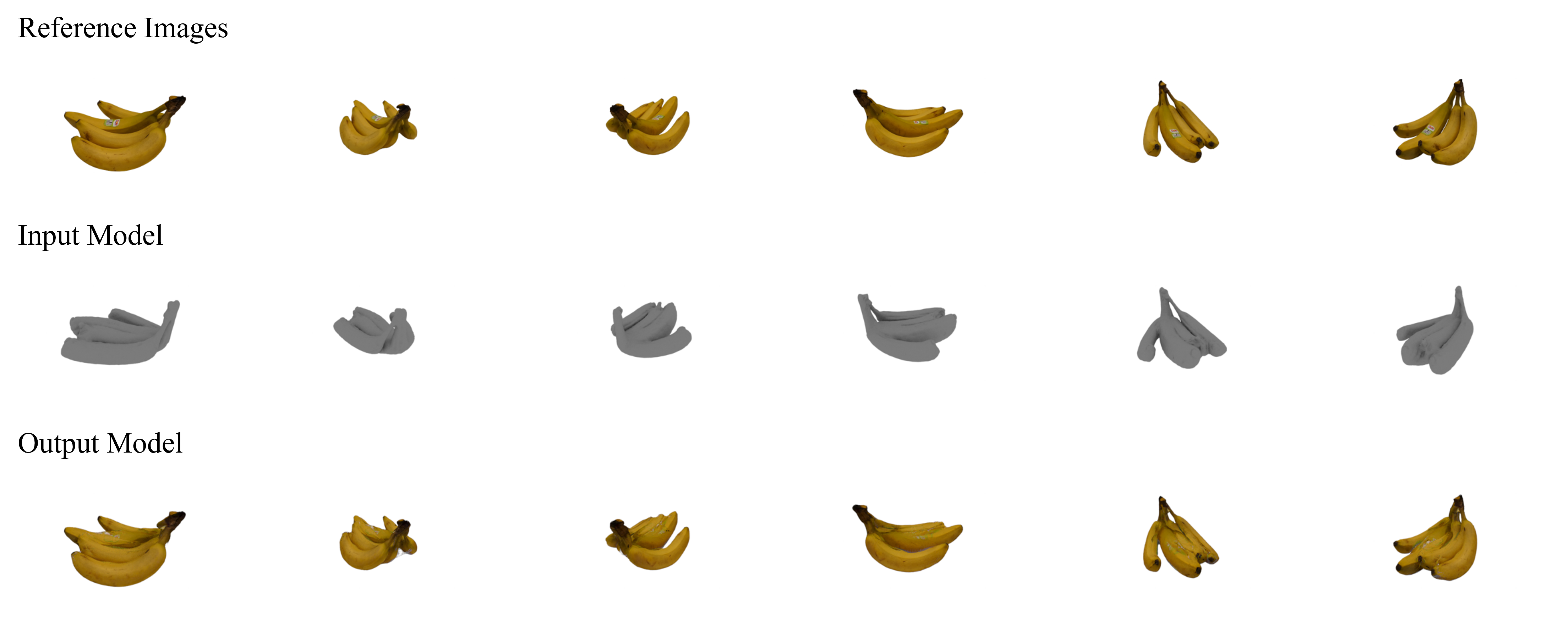
Figure 6: Optimization from the view-11 coarse mesh using six reference views.
Figure 7: Optimization from the same coarse mesh using all fourteen views.
The image-space metrics agree with the visual comparison:
| Initialization and training views | Average MSE ↓ | Average SSIM ↑ |
|---|---|---|
| Coarse view-11 mesh, 14 views | 0.0009 | 0.9735 |
| Coarse view-11 mesh, 6 views | 0.0013 | 0.9666 |
| Icosphere, 14 views | 0.0032 | 0.9547 |
| Icosphere, 6 views | 0.0059 | 0.9351 |
The 14-view coarse initialization reduces mean squared error by about 72% relative to the 14-view icosphere run. The improvement is even clearer when inspecting the mesh itself, because a low pixel error does not guarantee correct geometry.
The starting shape matters
To test whether the coarse reconstruction was genuinely useful, we repeated the optimization with a heavily subdivided icosphere while keeping every other parameter fixed. The naive initialization produced severe artifacts. Instead of moving the sphere into the correct shape, the optimizer often changed vertex colors to imitate the background, creating the appearance of the object’s silhouette from a training camera.
This is a useful failure mode: an optimizer will exploit any available degree of freedom. If geometry and color can both reduce the same pixel loss, color may become a shortcut for geometry. More views help, but they do not fully repair a poor initialization.
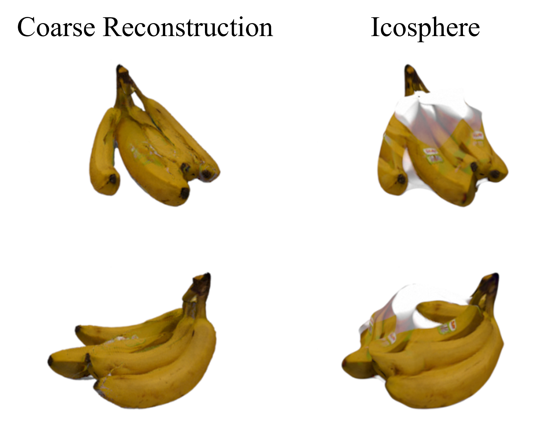
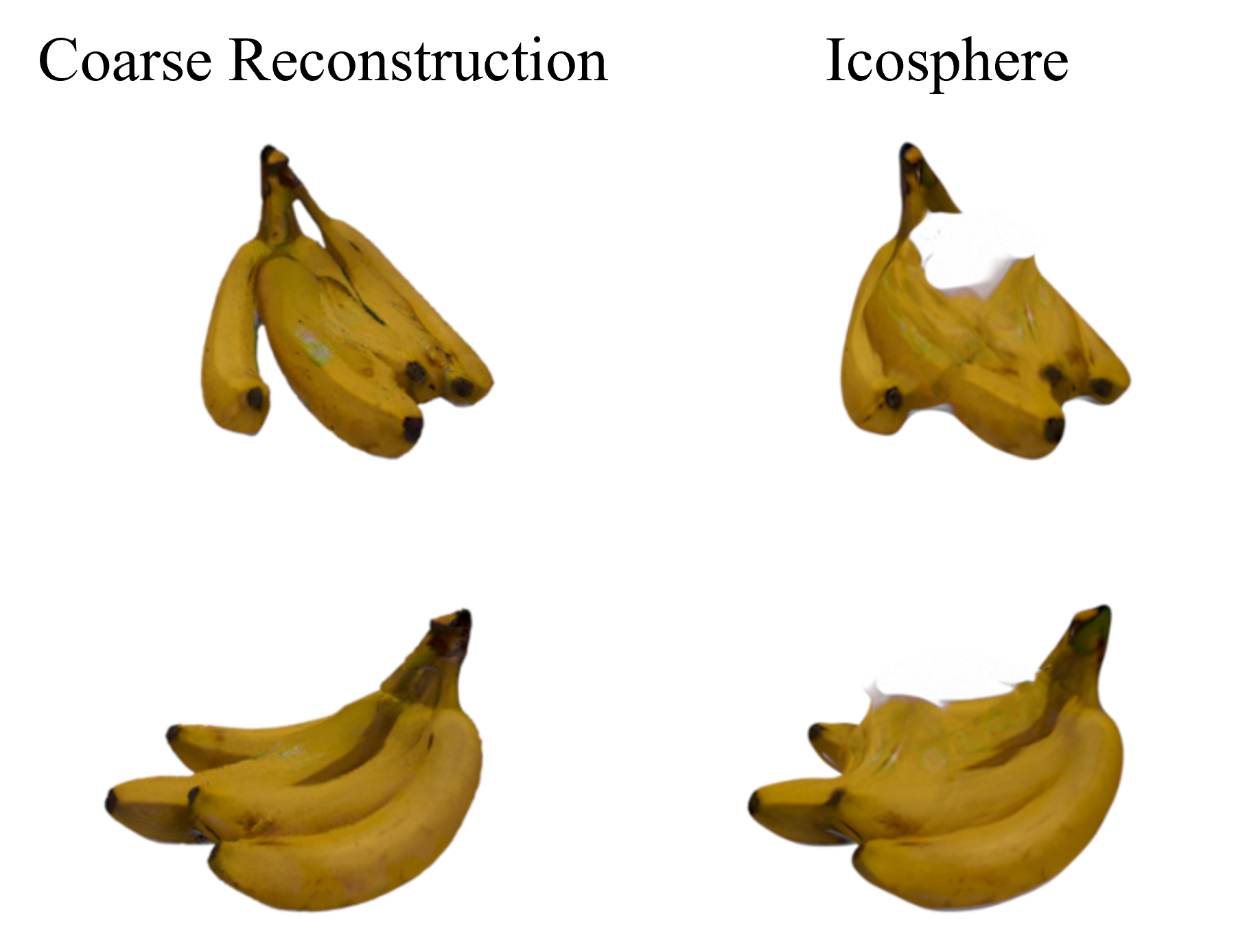
Figures 8–9: Coarse-mesh initialization versus an icosphere using six views (left) and fourteen views (right). Click either image to inspect it at full resolution.
The particular photograph used for single-image reconstruction matters too. View 11 showed the separation between individual bananas, while view 2 did not. Once TripoSR fused parts of the object, inverse rendering could refine the surface but could not reliably invent the missing topology.
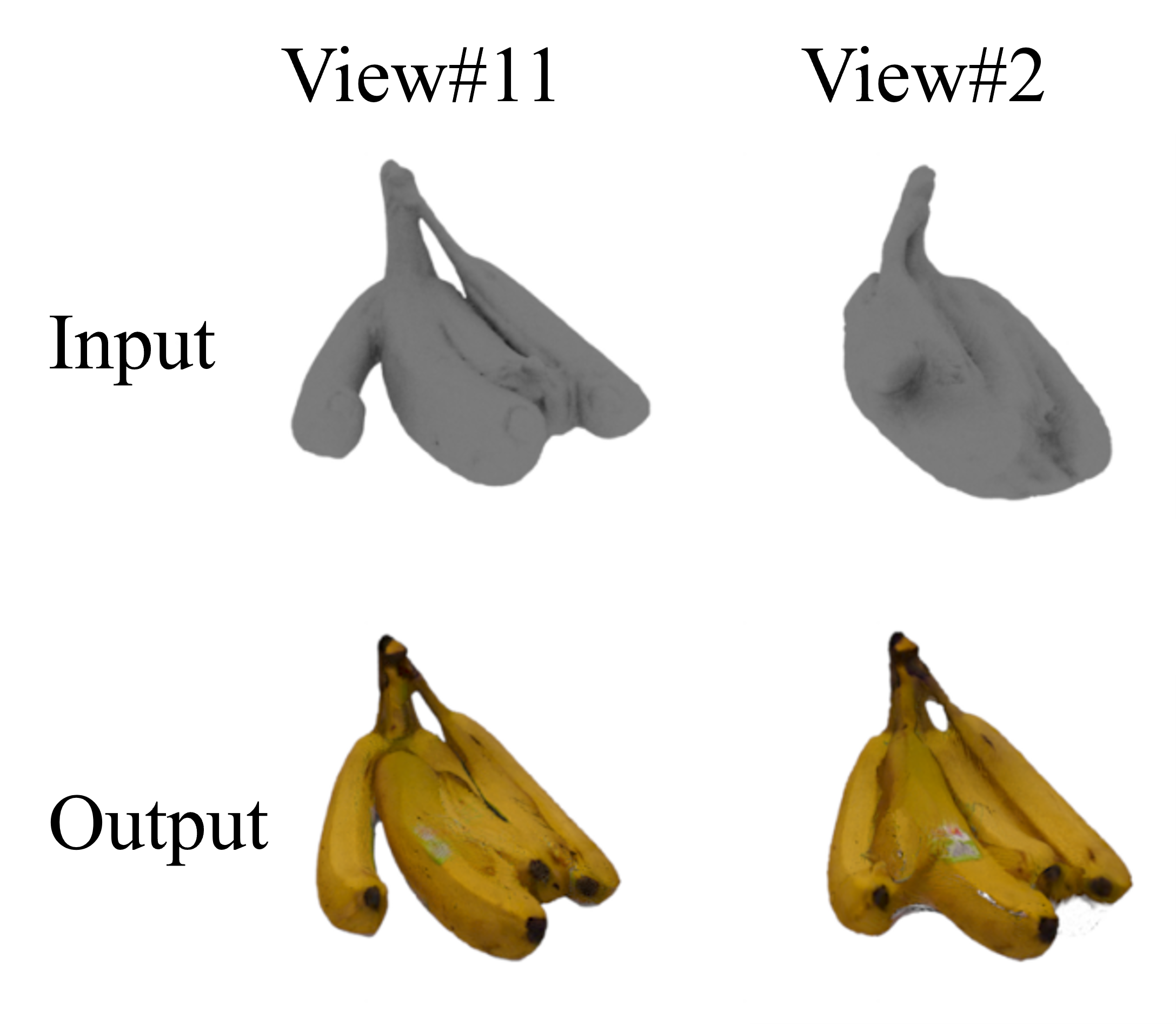
Figure 10: Coarse meshes produced from views 11 and 2, followed by their optimized results. Better visible topology in the source view leads to a better final mesh.
Performance
The early pipeline stages ran on an AMD Ryzen 5800X and NVIDIA RTX 3090. Inverse rendering was measured separately on an Intel Xeon Platinum 8358 virtual machine using Mitsuba’s LLVM backend. Median timings over five runs were:
| Stage | Observed time |
|---|---|
| COLMAP pose estimation for roughly 10 images | under 60 seconds |
| SAM 2 automatic segmentation | roughly 1 minute per megapixel |
| SAM 2 prompt-based segmentation and cleanup | under 30 seconds |
| TripoSR reconstruction and Marching Cubes | under 60 seconds |
| Inverse rendering with 6 views | 20–30 minutes |
| Inverse rendering with 14 views | about 1 hour |
The final stage dominates the runtime and scales roughly linearly with the number of views. Reducing the coarse mesh’s vertex count—and remeshing as the geometry evolves—would make the system much more practical.
What I would change next
The prototype validates the overall strategy, but it is not yet the seamless one-click system suggested by the diagram. Alignment and conversion between COLMAP, Blender, and Mitsuba still involve manual work. Automating that bridge is the clearest engineering improvement.
There are also several research directions worth exploring:
- optimize geometry before enabling vertex colors, or regularize color so it cannot hide silhouette errors;
- choose the coarse-reconstruction view automatically based on mask coverage and visible topology;
- add remeshing and reduce the initial vertex count to accelerate inverse rendering;
- test perceptual or silhouette-aware losses in addition to per-pixel L1;
- recover more expressive physically based materials and, eventually, the surrounding illumination.
The broader lesson is that the best reconstruction did not come from a single all-purpose method. It came from combining complementary priors: geometry for cameras, a segmentation foundation model for clean inputs, a learned model for plausible topology, and differentiable rendering for multi-view consistency. In this pipeline, the coarse mesh is not a disposable preview—it is the constraint that makes the final optimization behave like reconstruction rather than image imitation.